1. Particle Linear Depolarization Ratio Implementation
The most important improvement included in the SCC v4.0 is the implementation of a new optical product which is the particle linear depolarization ratio.
Important
If your lidar system is not equipped with any polarization channels NO changes are required. In this case, the SCC v4.0 should work using the same input files and the same database configurations you have used with the SCC v3.11. Anyway as in the SCC v4.0 several bugs have been fixed, it is recommended to re-run all the measurement IDs you have submitted. For doing that you just need to reprocess all your data without the need to submit raw data files already uploaded on the server.
1.1 Background
The calculation of the volume linear depolarization ratio profile (VLDR) and particle linear depolarization ratio profile (PLDR) needs two different steps:
- the calibration of the polarization sensitive lidar channels;
- the calculation of the VLDR or PLDR itself.
The SCC allows the user to make both the above points. In particular the calibration step is made by a completely new module called ELDEC (Earlinet Lidar Depolarization Calibrator) which computes the apparent calibration factor \(\eta^*\) out of the pre-processed data provided by the standard ELPP (Earlinet Lidar Pre-Processor) module and it records it in the SCC database (SCC_DB). Once logged into the SCC_DB this factor can be used whenever it is necessary.
The raw lidar calibration measurements should be put in a NetCDF file which has the same structure as the “standard” raw SCC NetCDF input file (for more details see sections 2 and 3.2).
New signal types have been introduced to take into account special channel configurations used for calibration purposes.
Moreover new product types for both calibration and PLDR calculation have been defined. As, in principle, it is possible to calculate the PLDR only when the aerosol backscatter coefficient profile is available the following new products have been defined:
- Linear polarization calibration (factor \(\eta\)) (product_type_id=6);
- Raman backscatter and linear depolarization ratio (product_type_id=7);
- Elastic backscatter and linear depolarization ratio (product_type_id=8).
The first product in the above list is used only for calibration while the other two are used for the calculation of PLDR. Basically, in most of the cases, the products 2 and 3 are equivalent to the corresponding backscatter product types with the exception that also the following new variables are available:
double VolumeDepol(Length) ;
double ErrorVolumeDepol(Length) ;
      ErrorVolumeDepol:long_name = "absolute error of VolumeDepol" ;
double ParticleDepol(Length) ;
double ErrorParticleDepol(Length) ;
      ErrorParticleDepol:long_name = "absolute error of ParticleDepol" ;
1.2 Polarization calibration
An important point is the definition of reliable PLDR calibration procedures. Within EARLINET the following calibration procedures are currently used:
- Rayleigh calibration;
- +45 calibration method, or \(\Delta90\) calibration method (made by +45 and -45 measurements);
- 3 signals (total, cross and parallel).
It is well known that method a) could produce easily large errors on PLDR which cannot be controlled. For this reason only the methods b) and c) can be used to provide reliable polarization calibrations and so only those methods will be implemented in the SCC.
For what it concerns the method c) it, basically, requires to solve the equation:
in two different atmospheric layers with considerably different VLDR. So to calibrate in this way the implementation of automatic layer identification in the SCC is required. As at moment this feature is not yet available within the SCC ONLY the method b) is considered.
1.3 SCC procedure to calculate the PLDRP
According to what mentioned before the SCC calculates the PLDR through the following steps:
- The user needs to create a new system configuration in the SCC_DB including only lidar channels used for the calibration. One (or more) Linear polarization calibration (product_type_id=6) product should be associated to this new configuration (see section 3.2 for more details);
- This new system configuration should contain only the polarization channels in the configuration used for the calibration (for example rotated in the polarization plane of +45 degrees). A channel in calibration measurement configuration should have a DIFFERENT channel ID from the channel ID corresponding to the same channel in standard measurement configuration. For example, if a system has two polarization channels which in standard measurement configuration correspond to the channel ID=1 and 2 respectively, the same physical channels under calibration measurement configuration should correspond to different channel IDs (let’s say ID=3 and 4 for the +45 degrees polarization rotated channels and ID=5 and 6 for the -45 degrees polarization rotated ones in case D90 calibration method is used). Moreover, the polarization channels should be labeled correctly using the new signal types available (+45elPT, +45elPR, -45elPT, -45elPR, +45elPTnr, +45elPTfr, +45elPRnr, +45elPRfr, -45elPTnr, -45elPTfr, -45elPRnr, -45elPRfr). For more details see section 3.2;
- In SCC v4.0 the polarization channels are NOT labeled on the base of their polarization state (as it was done in the SCC v3.11) but ALWAYS as transmitted and reflected channels. So the channels that in SCC v3.11 were labeled as elCP, elCPnr, elCPfr, elPP, elPPnr elPPfr will be labeled in SCC v4.0 as elPR, elPRnr elPRfr elPT, elPTnr elPTfr where the letter T stands from transmitted and the letter R for reflected.
Warning
- In switching from the SCC v3.11 to SCC v4.0 the following modifications have been made on ALL channels of ALL registered configurations:
elPP→elPR
elCP→elPT
elPPnr→elPRnr
elPPfr→ elPRfr
elCPnr→ elPTnr
elCPfr→ elPTfr
Please be sure these modifications reflect to your actual lidar setup(cross channels are transmitted and parallel channels are reflected);
- The user needs to submit a file (same format as raw SCC input file) containing the raw data for the lidar channels defined at the point 1 (see section 3.2 for more details);
- The file at point 4 is pre-processed by ELPP module which applies the standard pre-processing procedures applied to “standard” lidar data;
- The pre-processed files are then processed by the new modules ELDEC which calculates \(\eta^*\) the apparent calibration factor and logs it into the SCC_DB;
- The user needs to create a new system configuration in the SCC_DB (which should be different from the one used for the calibration) and associate it the new product Raman backscatter and linear depolarization ratio product_type_id=7) or Elastic backscatter and linear depolarization ratio (product_type_id=8). Alternatively the calculation of those products can be added to an already existing lidar configuration as long as it is different from the calibration one;
- The product defined at point 7 should be linked to the product containing the polarization calibration (defined at point 1) in a way that the apparent calibration factor can be selected from the SCC_DB (see section 3.3 and in particular figure 3.4);
- The user needs to submit another SCC raw data file containing the “standard” measurements;
- Finally ELPP and ELDA will produce a b-file containing backscatter coefficient profile and PLDR. In particular this calculation is made in two different steps: from the pre-processed lidar polarization signals, and taking into account the apparent calibration factor and the calibration factor correction K (defined as option of Linear polarization calibration product) written into the SCC_DB, an “apparent” VLDR \(\delta^*\) is calculated. Even if \(\delta^*\) is a calibrated quantity it can be still affected by possible systematic errors due to not perfect optics or alignment of the system;
- To take into account these errors a corrected VLDR (\(\delta\)) is calculated using the polarization cross-talk correction parameters G and H calculated on the base of Müller matrix formalism. These cross-talk correction parameters (G and H) are stored in the SCC_DB for each lidar channels (see section 3.1 in particular figure 3.2). Finally the PLDR is calculated using the backscatter coefficient profile and the molecular LDRP calculated by ELPP considering the center wavelength and bandwidth of the channels interference filter.
The apparent calibration factor \(\eta^*\) is calculated by the ELDEC module as the geometrical mean of the ratio of the +/-45 degrees reflected to the +/- 45 degrees transmitted signals within an altitude calibration range defined by the users in the raw data input files.
In case of +45 calibration method \(\eta^*\) is calculated by:
While in case of \(\Delta90\) calibration method:
ELDA module calculates the “apparent” VLDR:
the VLDR
and the PLDR
where:
- \(\eta^*\) is the apparent calibration factor calculated by ELDEC
- K is the calibration factor correction defined as polarization product option
- \(I_T\) and \(I_R\) are the transmitted and the reflected signals in the polarization detection set-up
- \(G_{T,R}\) and \(H_{T,R}\) are polarization cross-talk correction parameters for the transmitted and reflected signals used to correct for systematic errors. Both these factors are defined in the SCC_DB for each lidar channel.
- \(\delta_m\) is the molecular linear depolarization ratio calculated by ELPP
- R is the backscatter ratio
Please note once again that the polarization channels are described in terms of transmitted and reflected signals. This means that according to different lidar instrumental configurations, the transmitted or the reflected channel can contain total, perpendicular or parallel polarized signals.
In order to retrieve the backscatter profile the total signal must be obtained combining the transmitted and reflected polarized signals. The following formula is used:
The formulas above are general and can be adapted to all possible polarization lidar configurations selecting the right polarization cross-talk correction parameters (see Table 1.1).
Let’s suppose, for example, we have the perpendicular polarized lidar signal on the transmitted channel and the parallel polarized on reflected channel. For an ideal system (no diattenuation and cross-talk) we have:
If, on the other hand, we have the perpendicular polarized lidar signal on reflected channel and the total polarized on the transmitted for and ideal system we have:
Table 1.1: Polarization cross-talk correction parameters for ideal systems
| Laser polarization | Detected in lidar channel | |||
| Transmitted | Reflected | |||
| \(G_T\) | \(H_T\) | \(G_R\) | \(H_R\) | |
| total | 1 | 0 | 1 | 0 |
| parallel | 1 | 1 | 1 | 1 |
| cross | 1 | -1 | 1 | -1 |
The apparent calibration factor (\(\eta^*\)), the calibration factor correction (K) and the polarization cross-talk correction parameters are stored by ELPP module in the intermediate NetCDF files using the following variables:
Polarization_Channel_Gain_Factor(apparent calibration factor - \(\eta^*\) )Polarization_Channel_Gain_Factor_Correction(calib. factor corr. – K)G_TH_TG_RH_R
Finally new usecases have been defined to take into account all the possible lidar configurations. The details on that are provided as a separate file.
2. Changes of the SCC input format
The following minor changes have been applied to raw SCC data format:
The optional variable ID_Range has been REMOVED;
The OPTIONAL variable
int Signal_Type(channels)has been added. The possible values are the same available in the SCC_DB:0\(\rightarrow\)elT1\(\rightarrow\)elTnr2\(\rightarrow\)elTfr3\(\rightarrow\)vrRN24\(\rightarrow\)vrRN2nr5\(\rightarrow\)vrRN2fr6\(\rightarrow\)elPR7\(\rightarrow\)elPT8\(\rightarrow\)pRRlow9\(\rightarrow\)pRRhigh10\(\rightarrow\)elPRnr11\(\rightarrow\)elPRfr12\(\rightarrow\)elPTnr13\(\rightarrow\)elPTfr14\(\rightarrow\)vrRH2O15\(\rightarrow\)pRRhighnr16\(\rightarrow\)pRRhighfr17\(\rightarrow\)pRRlownr18\(\rightarrow\)pRRlowfr19\(\rightarrow\)vrRH2Onr20\(\rightarrow\)vrRH2Ofr21\(\rightarrow\)elTunr22\(\rightarrow\)+45elPT23\(\rightarrow\)+45elPR24\(\rightarrow\)-45elPT25\(\rightarrow\)-45elPR26\(\rightarrow\)+45elPTnr27\(\rightarrow\)+45elPTfr28\(\rightarrow\)+45elPRnr29\(\rightarrow\)+45elPRfr30\(\rightarrow\)-45elPTnr31\(\rightarrow\)-45elPTfr32\(\rightarrow\)-45elPRnr33\(\rightarrow\)-45elPRfrWarning
This variable is found in the SCC input file the corresponding settings in the SCC database will be OVERWRITTEN. Unless you don’t have any valid reason to overwrite the database value this variable should not be used.
The variables:
double Pol_Calib_Range_Min(channels)
double Pol_Calib_Range_Max(channels)
have been added. Both these variable are MANDATORY for any calibration raw dataset. These variable should be included only the polarization calibration measurements and should specify the altitude range (meters) in which the polarization calibration should be made. For more details see section 3.3;
- The variable
Depolarization_Factorhas been REMOVED.
The SCC v3.11 used this variable to get polarization calibration factor for the calculation of the total signal out of cross and parallels ones. As the SCC v4.0 is able to calculate the same parameter by itself, the use of this variable is NOT possible anymore. The recommended way to get a valid and quality assured depolarization calibration factor is to submit to the SCC v4.0 a polarization calibration dataset and let the SCC to calculate such factor.
To make this change more smooth and to provide the users with the possibility to continue to analyze their data with the SCC v4.0 even if a calibration dataset has not been submitted yet, it will be possible for a LIMITED period of time to submit the calibration constant via the SCC web interface. The SCC will keep track of the used calibration method (automatic or manual).
Warning
After this transition period ONLY automatic calibration will be allowed!
The new OPTIONAL variable:
string channel_string_ID(channels)
has been introduced.
Starting from SCC v4.0 the lidar channel can be identified not only by using integers (as it happened until SCC v3.11) but also by using strings.
The procedure implemented in the SCC v4.0 to recognize the lidar channel within the raw lidar data is fully backward compatible (old format files are accepted as they are by SCC v4.0).
Warning
Please note that the definition of the new string variable requires netCDF-4 format! The type string is not supported in netCDF-3 format!
3. Real Example
This section describes all the practical steps the users need to follow to switch from SCC v3.11 to new SCC v4.0.
| IMPORTANT: | If your lidar system is not equipped with any polarization channels NO changes are required. In this case, the SCC v4.0 should work using the same input files and the same database configurations you have used with the SCC v3.11. Anyway as in the SCC v4.0 several bugs have been fixed,it is recommended to re-run all the measurement IDs you have submitted. For doing that you just need to reprocess all your data without the need to submit raw data files already uploaded on the server. |
|---|
The practical example reported below describes the modifications required to use the SCC v4.0 for lidar systems equipped with polarization channels. Lidar systems not equipped with polarization channels do not require any modification to switch to SCC v4.0.
3.1 Modification of polarization channel parameters
In what it follows it is assumed you already have registered one or more lidar configurations in the SCC database and that such configurations have been already used to produce optical products (aerosol extinction and/or backscatter coefficients) by means of the SCC v3.11.
Let’s assume your 3+2 system is registered in the SCC database and the settings used by the SCC v3.11 are the ones summarized in table 3.1.
| Table 3.1: | Example of configuration in SCC v3.11 |
|---|
| Channel Name | Channel ID | Channel Type | nighttime | daytime |
| 355 | 1 | elT | x | x |
| 387 | 2 | vrRN2 | x | |
| 532 cross | 3 | elCP | x | x |
| 532 parallel | 4 | elPP | x | x |
| 607 | 5 | vrRN2 | x | |
| 1064 | 6 | elT | x | x |
We assume there are 2 system configurations called “nighttime” and “daytime”. The nighttime configuration contains all the available lidar channels (in order to calculate, for example, the aerosol extinction at 355 and 532nm and the aerosol backscatter at 355, 532 and 1064nm) while in daytime conditions only elastic channels are used (only elastic backscatter coefficients are generated).
To make these settings working with SCC v4.0 it is needed to modify :underline:ONLY` the products properties involving the polarization channels (532 cross and parallel). All the products not involving the polarization channels DO NOT need any modification and should work in the SCC v4.0 exactly as they did in SCC v3.11. In the example above the aerosol extinction and backscatter coefficient at 355nm, the extinction at 532nm as well as the backscatter coefficient at 1064nm do not required any modification. Let’s focus on the modifications needed for the calculation of backscatter at 532nm.
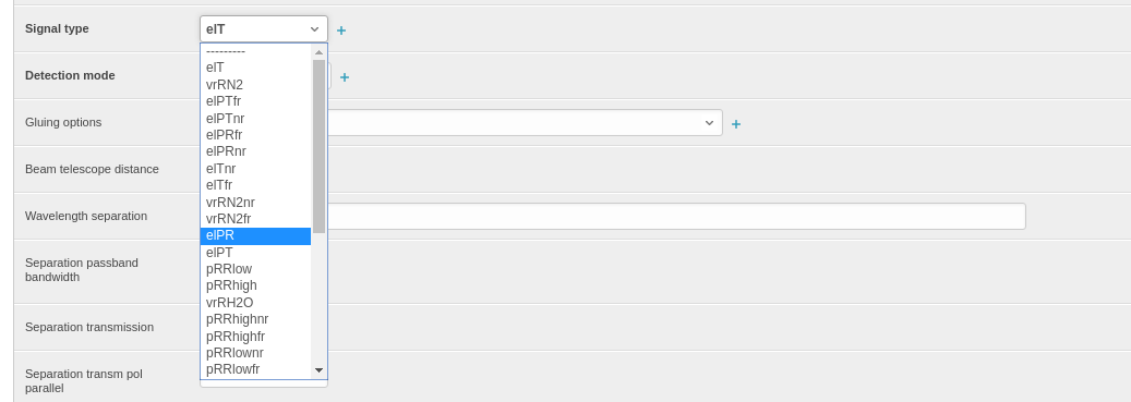
Figure 3.1: How to select signal types
The first modification concerns the settings of the channel type for the 532 cross and 532 parallel polarization channels. Starting from SCC v4.0 polarization channels are identified as transmitted and reflected polarization channels and not on the base of their polarization state. So if we suppose that the cross polarized channel is transmitted by a polarizer beam splitter cube, and the parallel is reflected, the value reported in table 3.1 should be modified as they appear in table 3.2. So using the SCC web interface, the signal type of the 532 cross channel should be changed from elCP to elPT and in the same way the 532 parallel channel should be changed from elPP to elPR (see figure 3.1).
Table 3.2: The same of table 3.1 but with new channel types introduced in SCC v4.0
| Channel Name | Channel ID | Channel Type | nighttime | daytime |
| 355 | 1 | elT | x | x |
| 387 | 2 | vrRN2 | x | |
| 532 cross | 3 | elPT | x | x |
| 532 parallel | 4 | elPR | x | x |
| 607 | 5 | vrRN2 | x | |
| 1064 | 6 | elT | x | x |
The other change about the polarization channels required to run the SCC v4.0 is the definition of the polarization crosstalk parameters for all the polarization channels available. Such parameters can be defined for each polarization channel using the SCC web interface (see figure 3.2). In particular among the channel parameters there is a new tab called Polarization crosstalk parameters where it is possible to insert the values from for the parameters G and H and the corresponding statistical and systematic errors if available. In case you have measured G and H for your polarization channels please insert the corresponding values there. Otherwise you can insert the ideal values as reported in table 1.1.
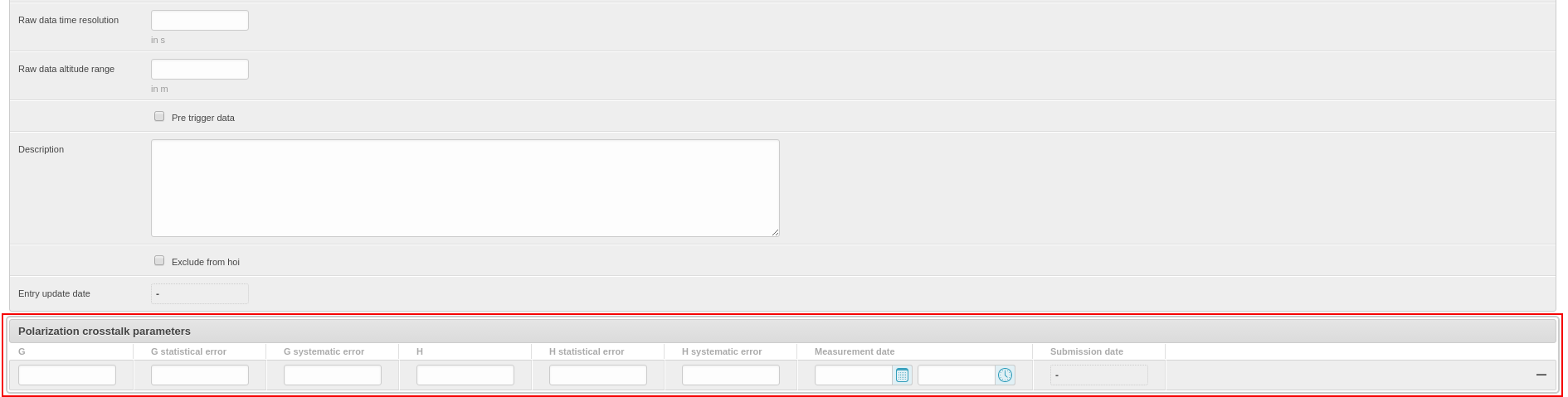
Figure 3.2: Polarization crosstalk parameters tab in channel properties (SCC v4.0).
3.2 Definition of new calibration configuration and product
In this section we will see how to set the polarization calibration parameters: the calibration constant (called \(\eta^*\) in section 1.3) and the correction to calibration constant (called K in section 1.3). In order to provide such parameters you need to define a new system configuration to be used ONLY for calibration purposes. Such new configuration should include the polarization channels in the measurement configuration used for the calibration. Let’s suppose we want to use the \(\Delta90\) calibration method.
In this case we need to define a new configuration (called for example “depol_calibration”) as reported in the table 3.3. As you can see the configuration “depol_calibration” includes 4 “new” channels. Actually the channels “532 cross +45 degrees” (channel ID=10) and “532 cross -45 degrees” (channel ID=12) refer to the same physical channel “532 cross” reported with channel ID=3 in table 3.2. Anyway we need to define two new channel IDs to identify the “532 cross” channel in the two polarization rotated configurations (+45 and -45 degrees) needed to apply the D90 calibration method. The same is true for the “532 parallel” channel. The polarization rotated channels should be labeled with the corresponding signal type as reported in table 3.3 (see figure 3.1).
Table 3.3: Polarization calibration configurations assuming \(\Delta90\) calibration method
| Channel Name | Channel ID | Channel Type | depol_calibration |
| 532 cross +45 degrees | 10 | +45elPT | x |
| 532 parallel +45 degrees | 11 | +45elPR | x |
| 532 cross -45 degrees | 12 | -45elPT | x |
| 532 parallel -45 degrees | 13 | -45elPR | x |
Finally we should add to the configuration “depol_calibration” a product “Linear polarization calibration” to be used for the calibration. According to the example given above and to the usecase document attached we should use an usecase=4 for this example.
Other “Linear polarization calibration” options to be specified are reported in figure 3.3. The most important factor you should insert here is the Pol calibration correction factor (K). The ideal value for this parameter is 1. Anyway if you have measured the parameter K please fill in the measured value and the corresponding measurement errors.
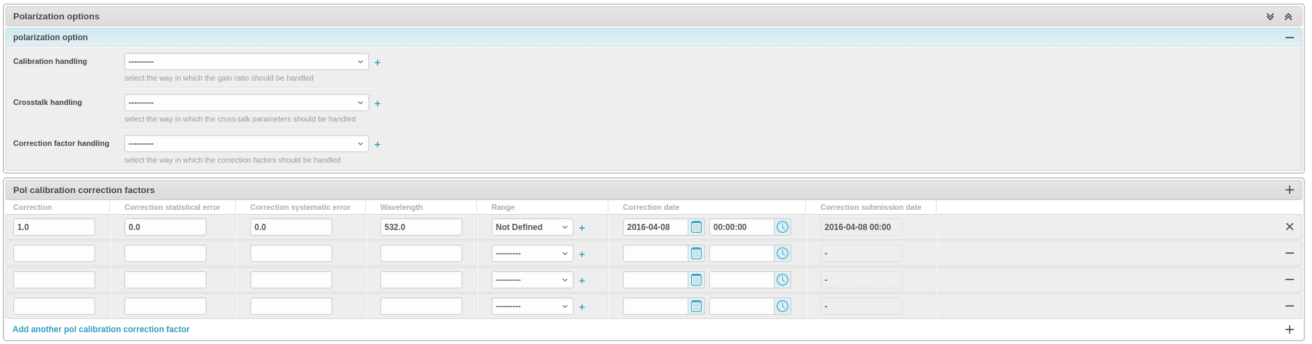
Figure 3.3: Options for Linear polarization calibration product.
As you can see it is possible to fill in only the K correction factor and not the calibration constant \(\eta^*\).
Actually for a LIMITED period of time it will be possible to fill in also the constant \(\eta^*\) using a temporary option shown in figure 3.4. This has been done to provide the users with the possibility to continue to use the SCC even if an automatic calibration made by the SCC was not submitted yet. Anyway after a transition period it will be NOT possible to provide calibration constant using this procedure and the parameter \(\eta^*\) can be calculated ONLY by the SCC as result of the submission of a proper calibration raw input dataset. The format of this input file is the same as the standard SCC input file. The only difference is that is should contain calibration measurements instead of standard measurements. Following our example, such file should contain the measurement performed at +45 and -45 degrees at 532nm. Also the channel IDs in the file should reflect the ones reported in table 3.3.
Moreover this raw input file has to contain the variables:
double Pol_Calib_Range_Min(channels)
double Pol_Calib_Range_Max(channels)
where to specify the altitude ranges in meters in which the polarization calibration should be done.
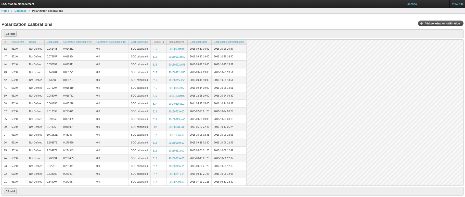
Figure 3.4: To provide polarization calibration (\(\eta^*\)) values manually just use the button “Add polarization calibration” in the upper-right corner. This option will be available only for a limited period of time. After that only SCC calculated calibration constants will be accepted.
According to the table 3.3 this file should be something similar to:
dimensions:
   channels = 4 ;
   nb_of_time_scales = 1 ;
   points = 16380 ;
   scan_angles = 1 ;
   time = UNLIMITED ; // (3 currently)
variables:
   int channel_ID(channels) ;
   double Background_Low(channels) ;
   double Background_High(channels) ;
   int id_timescale(channels) ;
   double Laser_Pointing_Angle(scan_angles) ;
   int Molecular_Calc ;
   int Laser_Pointing_Angle_of_Profiles(time, nb_of_time_scales) ;
   int Raw_Data_Start_Time(time, nb_of_time_scales) ;
   int Raw_Data_Stop_Time(time, nb_of_time_scales) ;
   int Laser_Shots(time, channels) ;
   double Raw_Lidar_Data(time, channels, points) ;
   double Pressure_at_Lidar_Station ;
   double Temperature_at_Lidar_Station ;
   double Pol_Calib_Range_Min(channels) ;
   double Pol_Calib_Range_Max(channels) ;

// global attributes:
         :System = "mysystem" ;
         :Longitude_degrees_east = 15.723771 ;
         :RawData_Start_Time_UT = "220000" ;
         :RawData_Start_Date = "20130620" ;
         :Measurement_ID = "20130620po00" ;
         :Altitude_meter_asl = 760. ;
         :RawData_Stop_Time_UT = "230333" ;
         :Latitude_degrees_north = 40.601039 ;

data:
 channel_ID = 10, 11, 12, 13 ;

 Background_Low = 30000, 30000, 30000, 30000 ;

 Background_High = 50000, 50000, 50000, 50000 ;

 id_timescale = 0, 0, 0, 0 ;

 Laser_Pointing_Angle = 0 ;

 Molecular_Calc = 0 ;

 Laser_Pointing_Angle_of_Profiles =
  0,
  0,
  0 ;

 Raw_Data_Start_Time =
  0,
  300,
  600 ;

 Raw_Data_Stop_Time =
  210,
  510,
  810 ;

 Laser_Shots =
  1200, 1200, 1200, 1200,
  1200, 1200, 1200, 1200,
  1200, 1200, 1200, 1200 ;

 Pressure_at_Lidar_Station = 1010 ;

 Temperature_at_Lidar_Station = 14 ;

 Pol_Calib_Range_Min = 1000, 1000, 1000, 1000 ;

 Pol_Calib_Range_Min = 2000, 2000, 2000, 2000 ;

 Raw_Lidar_Data = …...;
The file above assume the following calibration measurements have been done:
- First +45 degrees acquisition followed by a corresponding -45 degrees acquisition
- Measurement at +45 degrees
Start Time: 20130620 22:00:00
Stop Time: 20130620 22:01:00
Shots: 1200
- Measurement at -45 degrees
Start Time: 20130620 22:02:30
Stop Time: 20130620 22:03:30
Shots: 1200
- Second +45 degrees acquisition followed by a corresponding -45 degrees acquisition
- Measurement at +45 degrees
Start Time: 20130620 22:05:00
Stop Time: 20130620 22:06:00
Shots: 1200
- Measurement at -45 degrees
Start Time: 20130620 22:07:30
Stop Time: 20130620 22:08:30
Shots: 1200
- Third +45 degrees acquisition followed by a corresponding -45 degrees acquisition
- Measurement at +45 degrees
Start Time: 20130620 22:10:00
Stop Time: 20130620 22:11:00
Shots: 1200
- Measurement at -45 degrees
Start Time: 20130620 22:12:30
Stop Time: 20130620 22:13:30
Shots: 1200
As you can see there are 3 cycles of consecutive measurements at +45 and -45 degrees. That way the dimension time is set to 3.
The first +/-45 degrees measurement starts at “20130620 22:00:00” (start time of the first +45 measurement) and stops at “20130620 22:03:30” (stop time of the fist -45 measurement). As a consequence, according to the values of the global attributes RawData_Start_Date and RawData_Start_Time_UT we have to set:
Raw_Data_Start_Time[0]=0 (start of the first +45 measurement in
seconds since RawData_Start_Time_UT)
Raw_Data_Stop_Time[0]=210 (stop of the first -45 measurement in
seconds since RawData_Start_Time_UT)
Following a similar procedure for the other 2 cycles we have:
Raw_Data_Start_Time[1]=300 (start of the second +45 measurement in seconds since RawData_Start_Time_UT)
Raw_Data_Stop_Time[1]=510 (stop of the second -45 measurement in seconds since RawData_Start_Time_UT)
Raw_Data_Start_Time[2]=600 (start of the third +45 measurement in seconds since RawData_Start_Time_UT)
Raw_Data_Stop_Time[2]=810 (stop of the third -45 measurement in seconds since RawData_Start_Time_UT)
Moreover, according to the order of the channels in the channel_ID variable, the Raw_Lidar_Data array should be filled as it follows:
Raw_Lidar_Data[0][0][points] \(\rightarrow\) 1st measured transmitted signal at +45 degrees
Raw_Lidar_Data[0][1][points] \(\rightarrow\) 1st measured reflected signal at +45 degrees
Raw_Lidar_Data[0][2][points] \(\rightarrow\) 1st measured transmitted signal at -45 degrees
Raw_Lidar_Data[0][3][points] \(\rightarrow\) 1st measured reflected signal at -45 degrees
Raw_Lidar_Data[1][0][points] \(\rightarrow\) 2nd measured transmitted signal at +45 degrees
Raw_Lidar_Data[1][1][points] \(\rightarrow\) 2nd measured reflected signal at +45 degrees
Raw_Lidar_Data[1][2][points] \(\rightarrow\) 2nd measured transmitted signal at -45 degrees
Raw_Lidar_Data[1][3][points] \(\rightarrow\) 2nd measured reflected signal at -45 degrees
Raw_Lidar_Data[2][0][points] \(\rightarrow\) 3rd measured transmitted signal at +45 degrees
Raw_Lidar_Data[2][1][points] \(\rightarrow\) 3rd measured reflected signal at +45 degrees
Raw_Lidar_Data[2][2][points] \(\rightarrow\) 3rd measured transmitted signal at -45 degrees
Raw_Lidar_Data[2][3][points] \(\rightarrow\) 3rd measured reflected signal at -45 degrees
Once this file has been created it needs to be submitted to the SCC and linked to the configuration “depol_calibration”. The result of the SCC analysis on this file will be the calculation of the calibration constant h* that will be logged into the SCC database and can be used to calibrate Raman/Elastic backscatter products (see section 3.3).
3.3 Definition of “Raman/Elastic backscatter and linear depolarization ratio”
In order to calculate the PLDR we need to modify the polarization related products linked to the “standard” measurement configurations (the configuration called “nighttime” and/or “daytime” in table 3.2).
Let’s suppose we have defined the following products (defined already in SCC v3.11):
Table 3.4: Example of products configuration in SCC v3.11
| Product Name | Product ID | Product Type | nighttime | daytime |
Raman backscatter 355nm |
1 | Raman backscatter | x | |
Extinction 387nm |
2 | Extinction | x | |
Raman backscatter 532nm |
3 | Raman backscatter | x | |
Extinction 532nm |
4 | Extinction | x | |
Elastic backscatter 355nm |
5 | Elastic backscatter | x | |
Elastic backscatter 532nm |
6 | Elastic backscatter | x | |
Elastic backscatter 1064nm |
7 | Elastic backscatter | x | x |
Product ID=1, 2, 4, 5, 7 do not need any modification as they do not involve polarization channels. The only product that need to be modified are the Product ID=3 and 6. To produce b532 files containing also PLDR we need to modify the “nighttime” and “daytime” configurations to include a product of type “Raman backscatter and linear depolarization ratio” or “Elastic bakscatter and linear depolarization ratio” respectively. So the configuration reported in table 3.4 should be changed to match what is included in table 3.5.
Table 3.5: The same of table 3.4 but with new product types introduced in SCC v4.0
| Product Name | Product ID | Product Type | nighttime | daytime |
Raman backscatter 355nm |
1 | Raman backscatter | x | |
Extinction 387nm |
2 | Extinction | x | |
Raman backscatter 532nm |
10 | Raman backscatter and linear depolarization ratio | x | |
Extinction 532nm |
4 | Extinction | x | |
Elastic backscatter 355nm |
5 | Elastic backscatter | x | |
Elastic backscatter 532nm |
11 | Elastic backscatter and linear depolarization ratio | x | |
Elastic backscatter 1064nm |
7 | Elastic backscatter | x | x |
As you can see in table 3.5, the old product IDs=3 and 6 (present in table 3.4) have been replaced with the new product ID=10 and 11 to guarantee the calculation of PLDR.
It is important to set among the product options of the product ID=10 and 11 which calibration product we want to use for calibration (see section 3.2). This can be done using the SCC web interface setting the appropriate setting in the tab Polarization calibration products (see figure 3.4). According to the current example you should set here the calibration product defined in section 3.2.

Figure 3.5: How to link a product to calibrate with a calibration product.
Warning
Please note that also Raman/Elastic backscatter products need to be linked to a calibration product because the calibration constant and the corresponding correction factor is needed to calculate the total signal out of the two polarization components even if the PLDR is not involved in the product calculation.